The Robot-Tracking mode allows for seamless manipulation of the robot’s TCP (Tool Center Point) by simply moving and rotating the hand. This method provides the most intuitive way to control a robot with six degrees of freedom, eliminating the need for a teaching panel. Users can freely move around and focus solely on the positioning task.
Enabling the Robot-Tracking mode involves pressing and holding the middle finger against the thumb. Releasing the fingers instantly stops the robot’s movement. By utilizing straightforward hand gestures, the tracking speed can be easily adjusted to achieve either highly precise or rapid movements. The gripper can be controlled, as well, by pressing the index finger against the thumb for at least one second.
Robot Tracking Algorithm
The following section provides a comprehensive description of the tracking algorithm in detail.
The tracking algorithm can be divided into two main parts:
- Glove velocity estimation
- Glove angular velocity estimation
After properly scaling these states, they are transmitted to the robot. It’s important to mention that the robot’s speed is controlled, not its position. To estimate the above systems states, a 9-axis IMU mounted on the back of the hand is used.
Velocity Estimation
The block diagram illustrating the velocity estimation is presented below.

The velocity estimation of the glove uses linear accelerometer readings (excluding gravity) and orientation readings, which are directly provided by the IMU. The data is received at a sampling rate of 50Hz, but is subsequently downsampled to 10Hz to reduce computational complexity.
The first component in the process is the leveling correction block. It uses the orientation readings to transform the accelerometer data from the body frame back into the initial frame. This correction removes sensor misalignments and sloppy hand movements.
The corrected accelerometer vector is then passed through an integrator block, which calculates the velocity. Additionally, an estimation of the velocity error is subtracted to obtain the final corrected velocity. This step is crucial to counteract velocity drift that may occur within seconds due to accelerometer bias. Without correction, the velocity becomes unreliable and unusable.
The velocity error estimation is implemented using an error state Kalman filter. This filter leverages the knowledge that when the accelerometer readings fall below a certain threshold, the velocity should be close to zero too. By incorporating these pseudo measurements, the error state (consisting of acceleration and velocity error) is adjusted. The estimated velocity error closely reflects the drift present in the raw velocity. Subtracting this velocity error from the raw velocity results in a stable and reliable velocity estimate.
To mitigate minor movements, a threshold block is introduced, which sets the velocity to zero if it falls below a specific threshold. This ensures that only significant movements are considered.
The final step involves remapping the axis of the velocity vector to align with the robot’s axis. The remapped velocity is then transmitted to the robot for further use.
Results:
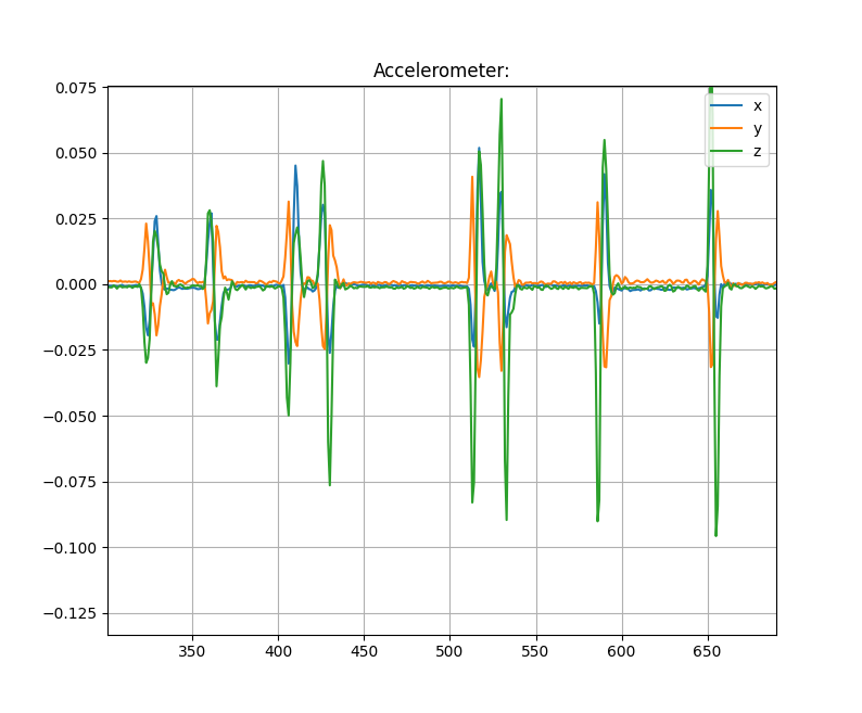
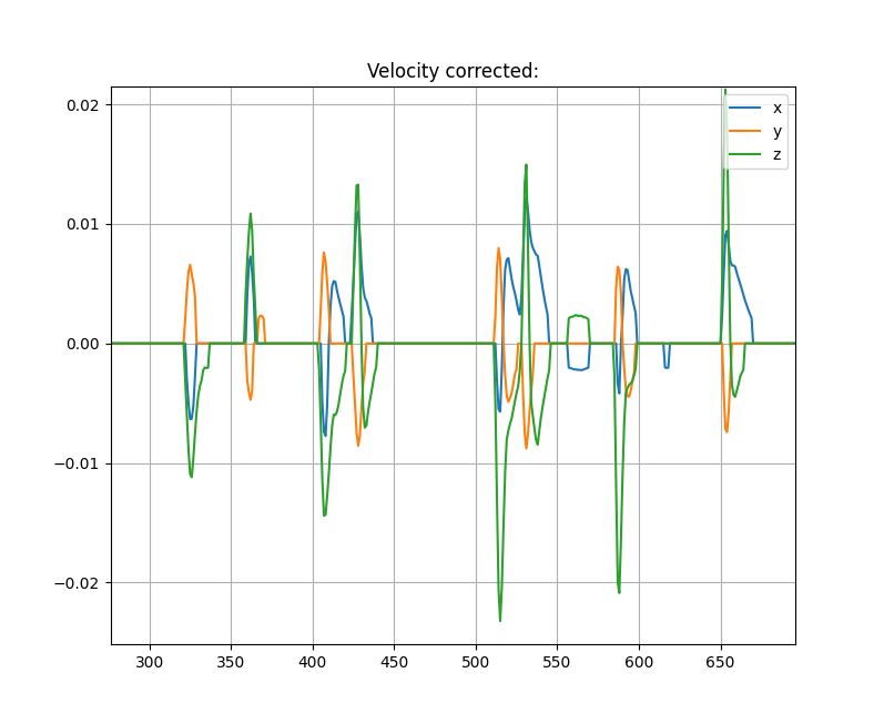
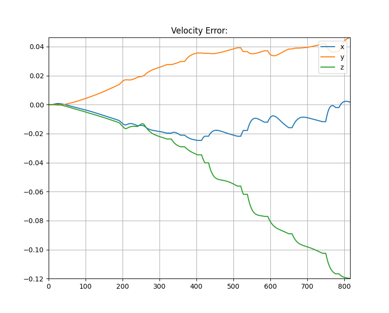
The gallery displays a collection of images showing examples of accelerometer readings, corrected velocity, and velocity error. In this particular example, the hand has been simultaneously moved along three axes, resulting in movement across all three axes.
Pay close attention to the significant increase in velocity error. It can clearly be seen that without correction, the velocity estimate is unusable within seconds. This emphasizes the importance of the correction process.
Please note that the x-axis of the images represents samples taken at a sampling rate of 10 Hz, while the y-axis is dimensionless.
Angular Velocity Estimation
The block diagram of the angular velocity estimation is presented below.

Compared to the velocity estimation, the process for angular velocity estimation is relatively straightforward.
The gyro readings, which represent angular velocity, are initially sampled at 50Hz and then downsampled to 10Hz, to reduce computational complexity.
To minimize high-frequency noise, a low-pass filter is applied. The filtered angular velocity values below a specific threshold are set to zero. This ensures that only significant angular movements are considered.
Next, the angular velocity vector is remapped to align with the robot’s axis once again, ensuring consistency in the coordinate system. Finally, the transformed vector is transmitted to the robot for further use.